Smart CFD – Can you get more for less?
Computational Fluid Dynamics (CFD) modelling is a proven tool for the analysis of real-world fluid flow and heat transfer problems, ranging from turbine blade design to fire and explosion assessment. To properly explore potential options or uncertainties may, however, require a large number of simulations, with the associated expansion of costs and timescales. So, is there a smarter way of unleashing the power of CFD?
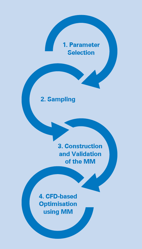
Figure 1 – 4 stages of meta model application
CFD-BASED OPTIMISATION
Computational Fluid Dynamics (CFD) has gained worldwide popularity due to its proven ability in design optimisation. Unlike physical testing, a large number of numerical simulations can be easily conducted with an arbitrarily low level of error.
However, the ever increasing sophistication and complexity of CFD models has led to higher computational costs, long model run times and the requirement for extensive user expertise. This is compounded by the increasing desire to vary more and more parameters in the search for optimised designs or a greater understanding of the effects of uncertainty, as an input to Quantitative Risk Assessment (QRA) for instance. Thankfully, there are smart methods available that can significantly reduce the CFD effort.
Over the last 70 years, Meta-Models (MMs) have gained wide adoption as a cost effective alternative to explicit modelling (Ref. 1). MMs (also known as multivariate interpolation / response surface methods) are a powerful tool for substantially reducing computational time and effort through the use of parametric input-output functions.
HOW IT WORKS
MMs allow the estimation of simulation results for a given set of input parameters, thus reducing the number of detailed simulations required. This is achieved through the 4 stage process shown in Figure 1.
MMs make predictions based on pre-prepared data from a limited set of complete CFD simulations. These simulations are chosen to cover variations in the required model parameters, with the parameter values appropriately sampled over the credible range in which they could fall.
Once the MM is trained and validated, the MM can be used in place of the CFD model for generating simulation results across the entire parameter-space (Ref. 3).

Figure 2 – Potential Sampling Schemes
DESIGN OF SAMPLING
Unfortunately, as the number of variables (or dimensions) increases, the number of CFD cases required increases exponentially. However, choosing an effective sampling method is a way to reduce the effect of increasing numbers of parameters (see Figure 2).
Available sampling techniques have various benefits and drawbacks, with the most commonly utilised methods being:
- Systematic Grid: This is the most basic sampling method, which utilises a grid of sample points splitting each parameter equally. This is, as it turns out, a very inefficient sampling method (this is clearer when considering 2D projections of the samples, since most of the points line up).
- Latin Hypercube Sampling: Another common sampling technique, which splits the domain into hypercubes and randomly places points. A drawback is that it does not guarantee adequate parameter-space filling.
- Quasi-Monte Carlo Sampling: Methods, such as Hammersley, Halton and Sobol sequences, were designed with efficient parameter-space filling in mind. Sobol sequences are the most efficient of these, and are generated based on primitive polynomials.
TRAINING AND VALIDATION
Prior to training the MM, any scale bias is removed by normalising each of the parameters. The model is trained using the combinations of parameter values generated by sampling and the corresponding CFD results. For testing purposes, a second set of random cases are generated together with CFD results.
The magnitude of errors is identified by comparing the MM values against the CFD results. The accuracy of predictions will vary based on a number of factors:
- Number of training data points
- Dimensionality of the data
- Distribution of training data points
- Whether the prediction points are within the domain defined by the training data
Example prediction surfaces and errors are shown in Figure 3.
There are multiple statistical techniques for determining the optimal trained model, such as the Coefficient of Determination (R²) and Likelihood Function. In practice, more than one technique should be used as there are limitations for each.
APPLICATIONS
MMs have been applied in some form in Explosion Risk Analysis (ERA) for the last 20 years (Ref. 2). Where this involves extensive and complex assets, plant and equipment, there is typically a need for a large number of simulations, given the wide range of possible release scenarios. Combinations of the input parameters can quickly result in thousands of dispersion simulations, simply by varying:
- Release rate, location and orientation
- Representative fluid (composition, temperature and pressure)
- Wind direction and speed
Similarly for explosions, the following variables might be considered:
- Gas cloud location, size and shape
- Representative fluid composition
- Ignition location
The use of MMs in this case can reduce the number of CFD simulations, but predictions can suffer from a loss of accuracy where consequences are especially sensitive to the parameters in question.
MMs can, however, be applied much more widely. Some known applications are listed below, along with the technique often used:
- Wind turbine blade design optimisation – Neural Networks, Genetic Aggregation Response
Surface (GARS) algorithm - Modelling CO2 leakage from a storage complex for CCS – Neural Networks, Gaussian Process Regression
- Reliability Analysis of Nuclear Passive Safety Systems – Genetic Aggregation Response Surface (GARS) algorithm, Neural Networks
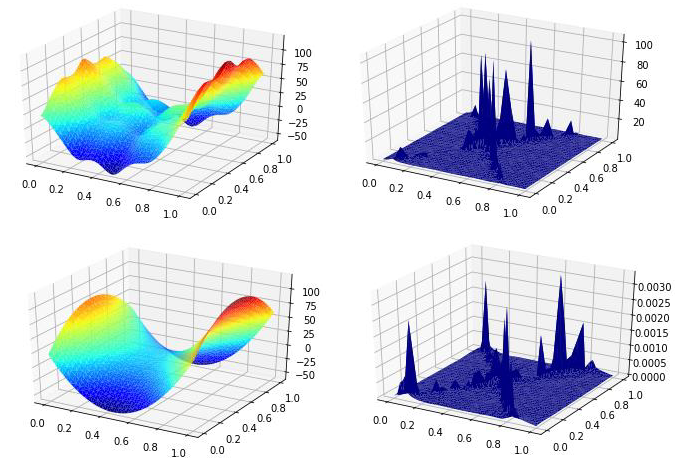
Figure 3 – Validation of Meta-Model
TOOLS
There are several commercially available tools for creating bespoke MMs; three of the most commonly used off the shelf include:
- Ansys Inc. Design Xplorer
- Stat-ease Inc. Design-Expert ®
- Mathworks Inc. Matlab
Choosing the correct MM has to consider:
- Accuracy of the results obtained
- Quality of the training database
- Volume of CFD calculations necessary to sufficiently train the model
- Extent to which the accuracy of predictions can be improved
COMPUTATIONAL POWER
Over the past two decades, microchip evolution has very closely followed Moore’s Law – the number of transistors on a microchip doubles every two years. Alongside the 1000-fold increase over this period, we have seen a significant increase in affordable computational power. This, in tandem with the ability to utilise high performance computing systems to run large numbers of simulations in a matter of days translates to greater accuracy and coverage of MMs. Conversely, we should not lose sight of the original motives for using MMs, and be aware that this same increase in computing power may dilute the benefits over explicit modelling in scenarios where the analysis cases are well defined.
CONCLUSION
MMs can substantially reduce computational time and effort when conducting CFD analysis with multiple variables, although some studies (such as ERA) are inherently less suited than others. This notwithstanding, the accuracy of the predictions are dependent on the sampling method, quality of the training data and choice of statistical
validation techniques.
Current applications of MMs range from physical effect modelling to reliability analysis. As computing power and speed continue their upward trajectory, the potential uses of MMs are probably only limited by our imagination.
This article first appeared in RISKworld 42, issued November 2022.
References
1. Box, G.E.P., 1951. Wilson. KB [1951] On the Experimental Attainment of Optimum Conditions. Journal of the Royal Statistical Society, Series B, 13(1), pp.1-45.
2. Huser, A., Eknes, M.L., Foyn, T.E., Selmer-Olsen, S. and Thevik, H.J., 2000. Express: Cost effective explosion risk management. In Major hazards offshore (London, 27-28 November 2000) (pp. 3-4).
3. Rößger, P. and Richter, A., 2018. Performance of different optimization concepts for reactive flow systems based on combined CFD and response surface methods. Computers & Chemical Engineering, 108, pp.232-239.