Divide and Conquer – Deriving structural failure probabilities using FE analysis
Many applications in mechanics require the consideration of uncertainty, and it can be useful to represent this uncertainty statistically, not least for informing probabilistic safety analysis or quantified risk assessment. However, with increasing complexity in system design and geometry, is there a practical method for deriving failure probabilities?
INTRODUCTION
Optimising structural form, so that a design can meet normal and extreme loads in an efficient way, requires a fundamental understanding of structural integrity, or rather the opposite – structural failure – in all its potential guises.
With the power of modern computational technology, the FE analysis method has become an essential part of structural analysis. Whether structures have mixed materials, diverse boundary conditions, time-dependent loadings, or nonlinear material behaviour, FE analysis is a proven technique for assessing structural integrity.
FE ANALYSIS 101
The core principle of FE analysis is partitioning a structure (such as a beam or a plate) into smaller, much simpler regions known as ‘finite elements’. Structures theory provides us with equations for each element in terms of its behaviour (e.g. stress and strain) under defined loads (e.g. point loads or pressure) and its interaction with immediately adjacent elements. All the equations can then be solved simultaneously to determine the behaviour of the structure as a whole, including the stress distribution (see Figure 1).
Whilst FE analysis is, without doubt, an excellent design tool, it is intrinsically deterministic – our structural FE model provides a definitive output, determined by our input data (model geometry, material properties, boundary conditions and loading).
In the real world, however, very little is certain. A designer will compensate for uncertainty by using conservative data – applying a corrosion allowance, pessimistic material properties, and bounding loadings – or by deliberately varying parameters to explore how influential they may be. But what if the same FE model could be repurposed to help us estimate the probability of structural failure?
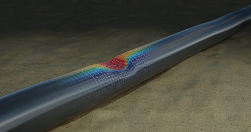
Figure 1 – 3D Pipeline Buckling Predicted by Finite Element Analysis
CHARACTERISING FAILURE
As with design, a crucial step on the road to probabilistic assessment is to define our failure criteria – relating perhaps to the ultimate limits of cracking, stretching (tension), compression, or plastic deformation. These failure criteria are defined on a best estimate basis, as opposed to the conservatism adopted during design, and are usually expressed as a ‘limit state function’. In basic terms, the limit state function is a measure of how far away a structure is from failure (e.g. the difference between the ultimate tensile stress and the imposed tensile stress).
To make analysis more tractable, we also want to limit the number of variables if we can. For this we can use the FE model directly to examine the effect that extreme values of a wide range of parameters might have on structural behaviour, discounting those that are of little influence.
ESTIMATING FAILURE PROBABILITY
Once left with a smaller handful of key parameters, the ideal would be to vary them all randomly according to their intrinsic probability distributions, using Monte Carlo simulation say, and feed each analysis case into the FE model to see whether failure occurs. If we did this 100,000 times and saw 2 failures, we would conclude that the probability of failure is 2E-5 for a given load demand. Unfortunately, while computing power has grown exponentially, approximately doubling every two years (Moore’s law), running a serious FE model 100,000 times is not economically viable if the answer is required in a useful timescale.
One alternative approach is to use a much more limited number of FE analysis cases (e.g. 100) to generate a ‘response surface’ for the limit state function across the key parameter space (see Figure 2). Whilst the details are quite technical, there are established methods, such as Sobol sampling, for producing a set of nicely spaced analysis cases; and Gaussian Process Regression, for achieving reasonable interpolative accuracy with relatively few known points. Some FE analysis software codes even include response surface modules, normally intended to aid design optimisation.
With our response surface defined, we can very rapidly interrogate it with an increasing number of randomly generated combinations of key parameters, looking for failures at every cycle and calculating the implied probability of failure until convergence is reached.
If failures are few, which might well be the case for conservatively designed structures, we can also validate the failures we see (or a sample of them) by further FE model runs, with results then used to update the response surface and our probabilistic predictions.
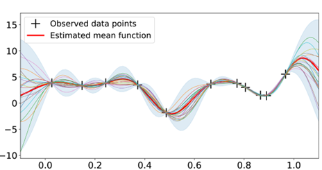
Figure 2 – Example of a Limit State Response Surface (reproduced from Ref. 1)
THE CHALLENGES
The beauty of this technique is that it makes use of a pre-existing FE model, which could otherwise be costly to develop, but it is not without its own challenges. First and possibly foremost is that it relies on defining the probability distributions of influential parameters. For material properties, this is normally straightforward, unless novel materials are proposed with sparse mechanical testing data.
More problematic can be defining loading probability distributions, which may be poorly characterised or may fluctuate with time. With respect to dynamic effects like this, it is important that the probability distribution is consistent with a specified unit of time – evaluating a frequency of failure per year, for example, requires a loading probability distribution for a year. Other challenges include:
- How to address geometrical variations in important design features caused by build tolerances in a way that minimises re-modelling time.
- Estimating the uncertainty in probability of failure evaluations, since not only does this require the definition of uncertainty of probability distributions themselves, but also greatly increases the number of randomised trials and the demand on computing time.
- Recording sufficient results data to support a meaningful and useful interpretation of results, while discarding other data to minimise data storage requirements.
On the last point, it is worth remembering that while computing the expected probability of failure is clearly of interest, it is as important to understand the most significant contributions to failure – i.e. the conditions, locations and failure modes – which may provide useful risk-related insights for the designer.
POTENTIAL APPLICATIONS
Nuclear power plant primary pipework and pressure vessels
Despite almost 160 years of study, there are still gaps in knowledge for predicting the probability of fatigue crack initiation under variable loading at high temperatures (Ref. 2). FE analysis-based defect tolerance and total-life approaches (the two main types of assessment) are typically employed for assessing high integrity components deterministically. Such models could also be used to provide complementary probabilistic assessment.
Seismic fragility analysis
While FE analysis is used extensively to understand and improve the response of structures in an earthquake, the estimation of the failure probability of key structures (termed fragility analysis) only makes use of the evaluated margin to failure, together with empirical definitions of uncertainty. Deploying FE models to support probabilistic analysis more directly could provide more relevant estimates or, alternatively, could help validate existing empirical approaches.
Carbon storage containment risk
Although projects involving the geological storage of CO2 can benefit from the insights provided by quantitative containment risk assessment, there is much uncertainty involved. Site-specific geomechanical FE models can, however, be re-used to characterise the probability of failure of key geological features, such as the primary seal and nearby faults (Ref. 3).
Wind turbine composite blade design optimisation
Composite materials are increasingly being used in industry, but there are numerous uncertainties around the fibre weaving and how this would behave on-site with variable wind conditions. As FE-based analysis tools are developed to address the unique properties of composites (e.g. Ref. 4), deploying them to make probabilistic failure predictions becomes a realistic prospect.
CONCLUSION
FE analysis is very often the design tool of choice for physical problems, including structural analysis. Until recently though, its application has, understandably, been limited to deterministic assessment. Where probabilistic assessment of integrity is also needed, however, the repurposing of an existing FE model to support Monte Carlo sampling of a response surface represents a practical, design-specific and cost-effective strategy, with potential applications we are only now beginning to appreciate.
References
- Jie Wang, An Intuitive Tutorial to Gaussian Process Regression, University of Waterloo, 2023. https://arxiv.org/html/2009.10862v5
- Prediction of fatigue crack initiation under variable amplitude loading: literature review. Metals, 13(3), p.487. Kedir, Y.A. and Lemu, H.G., 2023.
- SHARP Storage research project, https://www.sharp-storage-act.eu/
- D Müzel, S., Bonhin, E.P., Guimarães, N.M. and Guidi, E.S., 2020, Application of the finite element method in the analysis of composite materials: A review. Polymers, 12(4), p.818.